Introduction to Diffusion Models
This post aims to illustrate the core mathematical concepts in diffusion models neatly. You can also find the lecture notes I made, which are well-organized. If you use these slides, please cite this post:)
Note: This is highly based on Lil’Log and Ho et al. 2020.
Forward Diffusion Process
In a nutshell, diffusion models generate a sample in the dataset distribution from noise by learning the reverse process of the forward process consisting of injecting small noise into the images of the dataset.
We define a Markov chain of diffusion steps to slowly add small amount of Gaussian noise to a sample \(\mathbf{x}_0\) in \(T\) steps, producing a sequence of noisy samples \(\mathbf{x}_{1}, \ldots, \mathbf{x}_T\).
Definition: Forward Diffusion Process
\[q\left(\mathbf{x}_{t} \mid \mathbf{x}_{t-1}\right)=\mathcal{N}\left(\mathbf{x}_{t} ; \sqrt{1-\beta_{t}} \mathbf{x}_{t-1}, \beta_{t} \mathbf{I} \right) \quad q\left(\mathbf{x}_{1: T} \mid \mathbf{x}_{0}\right)=\prod_{t=1}^{T} q\left(\mathbf{x}_{t} \mid \mathbf{x}_{t-1}\right)\]where \(\mathbf{x}_0\) is a data point sampled from a real data distribution \(q(\mathbf{x}_0)\) and \(\left\{\beta_{t} \in(0,1)\right\}_{t=1}^{T}\) is a variance schedule.
Usually, we can afford a larger update step when the sample gets noisier, so \(\beta_{1}<\beta_{2}<\cdots<\beta_{T}\). Ho et al. 2020 set the forward process variances to constants increasing linearly from \(\beta_{1}=10^{-4}\) to \(\beta_{T}=0.02\).
Property 1
\[q\left(\mathbf{x}_{t} \mid \mathbf{x}_{0}\right)=\mathcal{N}\left(\mathbf{x}_{t} ; \sqrt{\bar{\alpha}_{t}} \mathbf{x}_{0},\left(1-\bar{\alpha}_{t}\right) \mathbf{I}\right)\]where \(\alpha_{t}=1-\beta_{t}\) and \(\bar{\alpha}_{t}=\prod_{i=1}^{t} \alpha_{i}\).
Proof)
\[\begin{array}{rlr} \mathbf{x}_{t} & =\sqrt{\alpha_{t}} \mathbf{x}_{t-1}+\sqrt{1-\alpha_{t}} \mathbf{z}_{t-1} ; \text { where } \mathbf{z}_{t-1}, \mathbf{z}_{t-2}, \cdots \sim \mathcal{N}(\mathbf{0}, \mathbf{I}) \\ & =\sqrt{\alpha_{t} \alpha_{t-1}} \mathbf{x}_{t-2}+\sqrt{1-\alpha_{t} \alpha_{t-1}} \overline{\mathbf{z}}_{t-2} \\ & \quad \text { where } \overline{\mathbf{z}}_{t-2} \text { merges two Gaussians }\\ & =\cdots \\ & =\sqrt{\bar{\alpha}_{t}} \mathbf{x}_{0}+\sqrt{1-\bar{\alpha}_{t}} \mathbf{\epsilon}_{t} ; \text{ where } \mathbf{\epsilon}_{t} \sim \mathcal{N}(\mathbf{0}, \mathbf{I})\\ q\left(\mathbf{x}_{t} \mid \mathbf{x}_{0}\right) & =\mathcal{N}\left(\mathbf{x}_{t} ; \sqrt{\bar{\alpha}_{t}} \mathbf{x}_{0},\left(1-\bar{\alpha}_{t}\right) \mathbf{I}\right) \quad \square \end{array}\]Eventually when \(T \rightarrow \infty, \mathbf{x}_{T}\) is equivalent to an isotropic Gaussian distribution.
Reverse Diffusion Process
The main idea is, “If we can reverse the above process and sample from \(q\left(\mathbf{x}_{t-1} \mid \mathbf{x}_{t}\right)\), we will be able to recreate the true sample from a Gaussian noise input, \({\mathbf{x}_{T} \sim \mathcal{N}(\mathbf{0}, \mathbf{I})}\).”
However, we cannot easily estimate \(q\left(\mathbf{x}_{t-1} \mid \mathbf{x}_{t}\right)\) because it needs to use the entire dataset. Therefore, we need to learn a model \(p_\theta\) to approximate these conditional probabilities!
Definition: Reverse Diffusion Process
Reverse Diffusion Process is defined as a Markov chain starting at \(p_{\theta}(\mathbf{x}_{T})=\mathcal{N}\left(\mathbf{x}_{T} ; \mathbf{0}, \mathbf{I}\right)\):
\[\begin{aligned} &p_{\theta}\left(\mathbf{x}_{t-1} \mid \mathbf{x}_{t}\right)=\mathcal{N}\left(\mathbf{x}_{t-1} ; \mathbf{\mu}_{\theta}\left(\mathbf{x}_{t}, t\right), \mathbf{\Sigma}_{\theta}\left(\mathbf{x}_{t}, t\right)\right)\\ &p_{\theta}\left(\mathbf{x}_{0: T}\right)=p_{\theta}\left(\mathbf{x}_{T}\right) \prod_{t=1}^{T} p_{\theta}\left(\mathbf{x}_{t-1} \mid \mathbf{x}_{t}\right) \end{aligned}\]Note that if \(\beta_t\) is small enough, \(q\left(\mathbf{x}_{t-1} \mid \mathbf{x}_{t}\right)\) is also Gaussian. Therefore, we define \(p_{\theta}\left(\mathbf{x}_{t-1} \mid \mathbf{x}_{t}\right)\) as a Gaussian distribution.
The overview of the forward and reverse process is illustrated in Fig. 1.
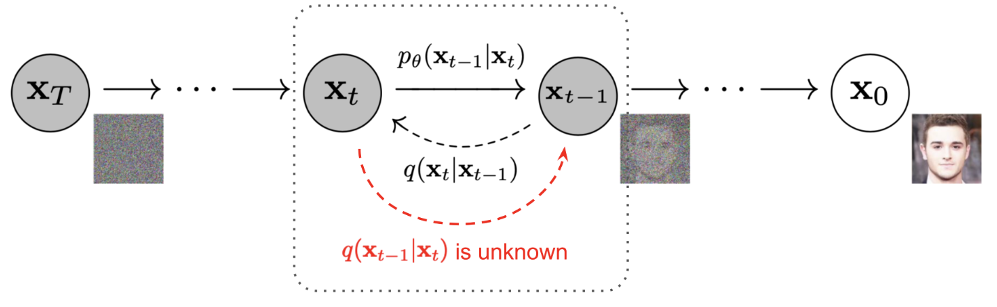 Fig. 1. Forward and reverse diffusion process. (Source: Lil’Log which is based on Ho et al. 2020)
Property 2
The reverse conditional probability \(q(\mathbf{x}_{t-1}\vert\mathbf{x}_t)\) is tractable when conditioned on \(\mathbf{x}_0\).
\[q\left(\mathbf{x}_{t-1} \mid \mathbf{x}_{t}, \mathbf{x}_{0}\right)=\mathcal{N}\left(\mathbf{x}_{t-1} ; \tilde{\mathbf{\mu}}_{t}\left(\mathbf{x}_{t}, \mathbf{x}_{0}\right), \tilde{\beta}_{t} \mathbf{I}\right)\]where \(\tilde{\mathbf{\mu}}_{t}\left(\mathbf{x}_{t}, \mathbf{x}_{0}\right)=\frac{\sqrt{\alpha_{t}}\left(1-\bar{\alpha}_{t-1}\right)}{1-\bar{\alpha}_{t}} \mathbf{x}_{t}+\frac{\sqrt{\bar{\alpha}_{t-1}} \beta_{t}}{1-\bar{\alpha}_{t}} \mathbf{x}_{0} = \frac{1}{\sqrt{\alpha_{t}}}\left(\mathbf{x}_{t}-\frac{\beta_{t}}{\sqrt{1-\bar{\alpha}_{t}}} \mathbf{\epsilon}_{t}\right)\) and \(\tilde{\beta}_{t}=\frac{1-\bar{\alpha}_{t-1}}{1-\bar{\alpha}_{t}} \cdot \beta_{t}\).
Proof)
\(* \text{ Gaussian PDF}: f(\mathbf{x}|\mathbf{\mu}, \mathbf{\Sigma}) = \operatorname{det}(2 \pi \mathbf{\Sigma})^{-\frac{1}{2}} \exp \left(-\frac{1}{2}(\mathbf{x}-\mathbf{\mu})^{\top} \mathbf{\Sigma}^{-1}(\mathbf{x}-\mathbf{\mu})\right)\) \(\begin{aligned} &q\left(\mathbf{x}_{t-1} \mid \mathbf{x}_{t}, \mathbf{x}_{0}\right) =q\left(\mathbf{x}_{t} \mid \mathbf{x}_{t-1}, \mathbf{x}_{0}\right) \frac{q\left(\mathbf{x}_{t-1} \mid \mathbf{x}_{0}\right)}{q\left(\mathbf{x}_{t} \mid \mathbf{x}_{0}\right)}=q\left(\mathbf{x}_{t} \mid \mathbf{x}_{t-1}\right) \frac{q\left(\mathbf{x}_{t-1} \mid \mathbf{x}_{0}\right)}{q\left(\mathbf{x}_{t} \mid \mathbf{x}_{0}\right)} \because \text{Markov} \\ & \propto \exp \left(-\frac{1}{2}\left(\frac{\left(\mathbf{x}_{t}-\sqrt{\alpha_{t}} \mathbf{x}_{t-1}\right)^{2}}{\beta_{t}}+\frac{\left(\mathbf{x}_{t-1}-\sqrt{\bar{\alpha}_{t-1}} \mathbf{x}_{0}\right)^{2}}{1-\bar{\alpha}_{t-1}}-\frac{\left(\mathbf{x}_{t}-\sqrt{\bar{\alpha}_{t}} \mathbf{x}_{0}\right)^{2}}{1-\bar{\alpha}_{t}}\right)\right) \\ &=\exp \left(-\frac{1}{2}\left(\left(\frac{\alpha_{t}}{\beta_{t}}+\frac{1}{1-\bar{\alpha}_{t-1}}\right) \mathbf{x}_{t-1}^{2}-\left(\frac{2 \sqrt{\alpha_{t}}}{\beta_{t}} \mathbf{x}_{t}+\frac{2 \sqrt{\bar{\alpha}_{t-1}}}{1-\bar{\alpha}_{t-1}} \mathbf{x}_{0}\right) \mathbf{x}_{t-1}+C\left(\mathbf{x}_{t}, \mathbf{x}_{0}\right)\right)\right) \end{aligned}\) where \(C\left(\mathbf{x}_{t}, \mathbf{x}_{0}\right)\) is a function not involving \(\mathbf{x}_{t-1}\).
\[\begin{flalign*} \tilde{\beta}_{t} &=1 /\left(\frac{\alpha_{t}}{\beta_{t}}+\frac{1}{1-\bar{\alpha}_{t-1}}\right)=\frac{1-\bar{\alpha}_{t-1}}{1-\bar{\alpha}_{t}} \cdot \beta_{t} \\ \tilde{\mathbf{\mu}}_{t}\left(\mathbf{x}_{t}, \mathbf{x}_{0}\right) &=\left(\frac{\sqrt{\alpha_{t}}}{\beta_{t}} \mathbf{x}_{t}+\frac{\sqrt{\bar{\alpha}_{t-1}}}{1-\bar{\alpha}_{t-1}} \mathbf{x}_{0}\right) /\left(\frac{\alpha_{t}}{\beta_{t}}+\frac{1}{1-\bar{\alpha}_{t-1}}\right)\\ &=\frac{\sqrt{\alpha_{t}}\left(1-\bar{\alpha}_{t-1}\right)}{1-\bar{\alpha}_{t}} \mathbf{x}_{t}+\frac{\sqrt{\bar{\alpha}_{t-1}} \beta_{t}}{1-\bar{\alpha}_{t}} \mathbf{x}_{0} \\ &=\frac{\sqrt{\alpha_{t}}\left(1-\bar{\alpha}_{t-1}\right)}{1-\bar{\alpha}_{t}} \mathbf{x}_{t}+\frac{\sqrt{\bar{\alpha}_{t-1}} \beta_{t}}{1-\bar{\alpha}_{t}} \frac{1}{\sqrt{\bar{\alpha}_{t}}}\left(\mathbf{x}_{t}-\sqrt{1-\bar{\alpha}_{t}} \mathbf{\epsilon}_{t}\right)\\ & \qquad \qquad \qquad \qquad \qquad \qquad \because \mathbf{x}_{0}=\frac{1}{\sqrt{\bar{\alpha}_{t}}}\left(\mathbf{x}_{t}-\sqrt{1-\bar{\alpha}_{t}} \mathbf{\epsilon}_{t}\right) \text{from Prop.1}\\ &=\frac{1}{\sqrt{\alpha_{t}}}\left(\mathrm{x}_{t}-\frac{\beta_{t}}{\sqrt{1-\bar{\alpha}_{t}}} \mathbf{\epsilon}_{t}\right) \quad \square && \end{flalign*}\]Learning Objective
Goal: We want to minimize the negative log-likelihood.
\[\begin{aligned} &\mathbb{E}_{\mathbf{x}_0 \sim q(\mathbf{x}_0)}\left[-\log p_{\theta}\left(\mathbf{x}_{0}\right)\right] \\ &\leq\mathbb{E}_{\mathbf{x}_0 \sim q(\mathbf{x}_0)}\left[-\log p_{\theta}\left(\mathbf{x}_{0}\right)+D_{\mathrm{KL}}\left(q\left(\mathbf{x}_{1: T} \mid \mathbf{x}_{0}\right) \| p_{\theta}\left(\mathbf{x}_{1: T} \mid \mathbf{x}_{0}\right)\right)\right]\\ &=\mathbb{E}_{\mathbf{x}_0 \sim q(\mathbf{x}_0)}\left[-\log p_{\theta}\left(\mathbf{x}_{0}\right)+\mathbb{E}_{\mathbf{x}_{1: T} \sim q\left(\mathbf{x}_{1: T} \mid \mathbf{x}_{0}\right)}\left[\log \frac{q\left(\mathbf{x}_{1: T} \mid \mathbf{x}_{0}\right)}{p_{\theta}\left(\mathbf{x}_{0: T}\right) / p_{\theta}\left(\mathbf{x}_{0}\right)}\right]\right] \\ &=\mathbb{E}_{\mathbf{x}_0 \sim q(\mathbf{x}_0)}\left[-\log p_{\theta}\left(\mathbf{x}_{0}\right)+\mathbb{E}_{\mathbf{x}_{1: T} \sim q\left(\mathbf{x}_{1: T} \mid \mathbf{x}_{0}\right)}\left[\log \frac{q\left(\mathbf{x}_{1: T} \mid \mathbf{x}_{0}\right)}{p_{\theta}\left(\mathbf{x}_{0: T}\right)}+\log p_{\theta}\left(\mathbf{x}_{0}\right)\right]\right] \\ &=\mathbb{E}_{\mathbf{x}_{0:T} \sim q(\mathbf{x}_{0: T})}\left[\log \frac{q\left(\mathbf{x}_{1: T} \mid \mathbf{x}_{0}\right)}{p_{\theta}\left(\mathbf{x}_{0: T}\right)}\right] := L_{\mathrm{VLB}} \end{aligned}\]In other words, we can achieve the goal by minimizing \(L_{\mathrm{VLB}}\)!
Remark 1: \(L_{\mathrm{VLB}}\)
We can convert \(L_{\mathrm{VLB}}\) to be analytically computable.
\[\begin{aligned} L_{\mathrm{VLB}}=&\mathbb{E}_{q(\mathbf{x}_0)}[\underbrace{D_{\mathrm{KL}}\left(q\left(\mathbf{x}_{T} \mid \mathbf{x}_{0}\right) \| p_{\theta}\left(\mathbf{x}_{T}\right)\right)}_{L_{T}}]\\ &+\sum_{t=2}^{T} \mathbb{E}_{q(\mathbf{x}_0, \mathbf{x}_t)}[\underbrace{D_{\mathrm{KL}}\left(q\left(\mathbf{x}_{t-1} \mid \mathbf{x}_{t}, \mathbf{x}_{0}\right) \| p_{\theta}\left(\mathbf{x}_{t-1} \mid \mathbf{x}_{t}\right)\right)}_{L_{t-1}}] \\ &+\mathbb{E}_{q(\mathbf{x}_0, \mathbf{x}_1)}[\underbrace{-\log p_{\theta}\left(\mathbf{x}_{0} \mid \mathbf{x}_{1}\right)}_{L_0}] \end{aligned}\]proof)
\[\begin{flalign*} &L_{\mathrm{VLB}}=\mathbb{E}_{q\left(\mathbf{x}_{0: T}\right)}\left[\log \frac{q\left(\mathbf{x}_{1: T} \mid \mathbf{x}_{0}\right)}{p_{\theta}\left(\mathbf{x}_{0: T}\right)}\right] \\ &=\mathbb{E}_{q}\left[\log \frac{\prod_{t=1}^{T} q\left(\mathbf{x}_{t} \mid \mathbf{x}_{t-1}\right)}{p_{\theta}\left(\mathbf{x}_{T}\right) \prod_{t=1}^{T} p_{\theta}\left(\mathbf{x}_{t-1} \mid \mathbf{x}_{t}\right)}\right]\\ &=\mathbb{E}_{q}\left[-\log p_{\theta}\left(\mathbf{x}_{T}\right)+\sum_{t=1}^{T} \log \frac{q\left(\mathbf{x}_{t} \mid \mathbf{x}_{t-1}\right)}{p_{\theta}\left(\mathbf{x}_{t-1} \mid \mathbf{x}_{t}\right)}\right]\\ &=\mathbb{E}_{q}\left[-\log p_{\theta}\left(\mathbf{x}_{T}\right)+\sum_{t=2}^{T} \log \frac{q\left(\mathbf{x}_{t} \mid \mathbf{x}_{t-1}\right)}{p_{\theta}\left(\mathbf{x}_{t-1} \mid \mathbf{x}_{t}\right)}+\log \frac{q\left(\mathbf{x}_{1} \mid \mathbf{x}_{0}\right)}{p_{\theta}\left(\mathbf{x}_{0} \mid \mathbf{x}_{1}\right)}\right]\\ &=\mathbb{E}_{q}\left[-\log p_{\theta}\left(\mathbf{x}_{T}\right)+\sum_{t=2}^{T} \log \left(\frac{q\left(\mathbf{x}_{t-1} \mid \mathbf{x}_{t}, \mathbf{x}_{0}\right)}{p_{\theta}\left(\mathbf{x}_{t-1} \mid \mathbf{x}_{t}\right)} \cdot \frac{q\left(\mathbf{x}_{t} \mid \mathbf{x}_{0}\right)}{q\left(\mathbf{x}_{t-1} \mid \mathbf{x}_{0}\right)}\right)+\log \frac{q\left(\mathbf{x}_{1} \mid \mathbf{x}_{0}\right)}{p_{\theta}\left(\mathbf{x}_{0} \mid \mathbf{x}_{1}\right)}\right] \\ & \qquad \qquad \qquad \qquad \qquad \qquad \qquad \qquad \qquad \qquad \qquad \because \text{Markov property and Bayes' rule} \\ &=\mathbb{E}_{q}\left[-\log p_{\theta}\left(\mathbf{x}_{T}\right)+\sum_{t=2}^{T} \log \frac{q\left(\mathbf{x}_{t-1} \mid \mathbf{x}_{t}, \mathbf{x}_{0}\right)}{p_{\theta}\left(\mathbf{x}_{t-1} \mid \mathbf{x}_{t}\right)}+\sum_{t=2}^{T} \log \frac{q\left(\mathbf{x}_{t} \mid \mathbf{x}_{0}\right)}{q\left(\mathbf{x}_{t-1} \mid \mathbf{x}_{0}\right)}+\log \frac{q\left(\mathbf{x}_{1} \mid \mathbf{x}_{0}\right)}{p_{\theta}\left(\mathbf{x}_{0} \mid \mathbf{x}_{1}\right)}\right]\\ &=\mathbb{E}_{q}\left[-\log p_{\theta}\left(\mathbf{x}_{T}\right)+\sum_{t=2}^{T} \log \frac{q\left(\mathbf{x}_{t-1} \mid \mathbf{x}_{t}, \mathbf{x}_{0}\right)}{p_{\theta}\left(\mathbf{x}_{t-1} \mid \mathbf{x}_{t}\right)}+\log \frac{q\left(\mathbf{x}_{T} \mid \mathbf{x}_{0}\right)}{q\left(\mathbf{x}_{1} \mid \mathbf{x}_{0}\right)}+\log \frac{q\left(\mathbf{x}_{1} \mid \mathbf{x}_{0}\right)}{p_{\theta}\left(\mathbf{x}_{0} \mid \mathbf{x}_{1}\right)}\right]\\ &=\mathbb{E}_{q}\left[\log \frac{q\left(\mathbf{x}_{T} \mid \mathbf{x}_{0}\right)}{p_{\theta}\left(\mathbf{x}_{T}\right)}+\sum_{t=2}^{T} \log \frac{q\left(\mathbf{x}_{t-1} \mid \mathbf{x}_{t}, \mathbf{x}_{0}\right)}{p_{\theta}\left(\mathbf{x}_{t-1} \mid \mathbf{x}_{t}\right)}-\log p_{\theta}\left(\mathbf{x}_{0} \mid \mathbf{x}_{1}\right)\right]\\ &=\mathbb{E}_{q(\mathbf{x}_0)}[\underbrace{D_{\mathrm{KL}}\left(q\left(\mathbf{x}_{T} \mid \mathbf{x}_{0}\right) \| p_{\theta}\left(\mathbf{x}_{T}\right)\right)}_{L_{T}}] +\sum_{t=2}^{T} \mathbb{E}_{q(\mathbf{x}_0, \mathbf{x}_t)}[\underbrace{D_{\mathrm{KL}}\left(q\left(\mathbf{x}_{t-1} \mid \mathbf{x}_{t}, \mathbf{x}_{0}\right) \| p_{\theta}\left(\mathbf{x}_{t-1} \mid \mathbf{x}_{t}\right)\right)}_{L_{t-1}}] \\ & \quad +\mathbb{E}_{q(\mathbf{x}_0, \mathbf{x}_1)}[\underbrace{-\log p_{\theta}\left(\mathbf{x}_{0} \mid \mathbf{x}_{1}\right)}_{L_0}] && \end{flalign*}\]Definition: \(L_T\), \(L_{t-1}\), and \(L_0\)
\[\begin{aligned} &(1) \, L_{T} =D_{\mathrm{KL}}\left(q\left(\mathbf{x}_{T} \mid \mathbf{x}_{0}\right) \| p_{\theta}\left(\mathbf{x}_{T}\right)\right) \\ &(2) \, L_{t-1} =D_{\mathrm{KL}}\left(q\left(\mathbf{x}_{t-1} \mid \mathbf{x}_{t}, \mathbf{x}_{0}\right) \| p_{\theta}\left(\mathbf{x}_{t-1} \mid \mathbf{x}_{t}\right)\right) \text { for } 2 \leq t \leq T \\ &(3) \, L_{0} =-\log p_{\theta}\left(\mathbf{x}_{0} \mid \mathbf{x}_{1}\right) \end{aligned}\]1) \(L_T\)
\(\quad \bullet\) From Prop.1, \(q\left(\mathbf{x}_{T} \mid \mathbf{x}_{0}\right) \rightarrow \mathcal{N}\left(\mathbf{x}_{T} ; \mathbf{0}, \mathbf{I}\right)\) when \(T \rightarrow \infty\).
\(\quad \bullet\) We assume that \(p_{\theta}(\mathbf{x}_{T})=\mathcal{N}\left(\mathbf{x}_{T} ; \mathbf{0}, \mathbf{I}\right)\).
\(\quad \bullet\) \(L_T\) is constant and can be ignored during training.
2) \(L_{t-1}\)
\(\quad \bullet\) This term measures the difference between \(q\left(\mathbf{x}_{t-1} \mid \mathbf{x}_{t}, \mathbf{x}_{0}\right)\) and \(p_{\theta}\left(\mathbf{x}_{t-1} \mid \mathbf{x}_{t}\right)\).
\(\quad \bullet\) How do we optimize this term? (Explained below)
3) \(L_0\)
\(\quad \bullet\) This term reconstruct the original image from the slightly noised image.
\(\quad \bullet\) This term is optimized by MSE loss: \(\left\|\mathbf{x}_{0}-\mathbf{\mu}_{\theta}\left(\mathbf{x}_{1}, 1\right)\right\|^{2}\)
How to optimize \(L_{t-1}\)
\(L_{t-1} =D_{\mathrm{KL}}\left(q\left(\mathbf{x}_{t-1} \mid \mathbf{x}_{t}, \mathbf{x}_{0}\right) \| p_{\theta}\left(\mathbf{x}_{t-1} \mid \mathbf{x}_{t}\right)\right)\)
\(q\left(\mathbf{x}_{t-1} \mid \mathbf{x}_{t}, \mathbf{x}_{0}\right)=\mathcal{N}\left(\mathbf{x}_{t-1} ; \tilde{\mathbf{\mu}}_{t}\left(\mathbf{x}_{t}, \mathbf{x}_{0}\right), \tilde{\beta}_{t} \mathbf{I}\right) = \mathcal{N}\left(\mathbf{x}_{t-1} ; \frac{1}{\sqrt{\alpha_{t}}}\left(\mathbf{x}_{t}-\frac{\beta_{t}}{\sqrt{1-\bar{\alpha}_{t}}} \mathbf{\epsilon}_{t}\right), \frac{1-\bar{\alpha}_{t-1}}{1-\bar{\alpha}_{t}} \beta_{t}\mathbf{I}\right)\)
\(p_{\theta}\left(\mathbf{x}_{t-1} \mid \mathbf{x}_{t}\right)=\mathcal{N}\left(\mathbf{x}_{t-1} ; \mathbf{\mu}_{\theta}\left(\mathbf{x}_{t}, t\right), \mathbf{\Sigma}_{\theta}\left(\mathbf{x}_{t}, t\right)\right)\)
Let us set \(\mathbf{\mu}_{\theta}\left(\mathbf{x}_{t}, t\right)=\frac{1}{\sqrt{\alpha_{t}}}\left(\mathbf{x}_{t}-\frac{\beta_{t}}{\sqrt{1-\bar{\alpha}_{t}}} \mathbf{\epsilon}_{\theta}(\mathbf{x}_{t}, t)\right)\) and \(\mathbf{\Sigma}_{\theta}\left(\mathbf{x}_{t}, t\right) = \sigma_{t}^{2}\mathbf{I}\).
We have two options for \(\sigma_{t}^{2}\): \(\sigma_{t}^{2}=\beta_{t}\) and \(\sigma_{t}^{2}=\frac{1-\bar{\alpha}_{t-1}}{1-\bar{\alpha}_{t}} \beta_{t}\).
According to Ho et al. 2020, both had similar results experimentally.
\(* D_{K L}(p \| q)=\frac{1}{2}\left[\log \frac{\left|\Sigma_{q}\right|}{\left|\Sigma_{p}\right|}-k+\left(\mathbf{\mu}_{p}-\mathbf{\mu}_{q}\right)^{T} \Sigma_{q}^{-1}\left(\mathbf{\mu}_{p}-\mathbf{\mu}_{q}\right)+\operatorname{tr}\left\{\Sigma_{q}^{-1} \Sigma_{p}\right\}\right]\) \(\begin{aligned} L_{t-1} &\propto \frac{1}{2\sigma_{t}^{2}}\left\|\tilde{\mathbf{\mu}}_{t}\left(\mathbf{x}_{t}, \mathbf{x}_{0}\right)-\mathbf{\mu}_{\theta}\left(\mathbf{x}_{t}, t\right)\right\|^{2}\\ &=\frac{1}{2\sigma_{t}^{2}}\left\|\frac{1}{\sqrt{\alpha_{t}}}\left(\mathbf{x}_{t}-\frac{\beta_{t}}{\sqrt{1-\bar{\alpha}_{t}}} \mathbf{\epsilon}_{t}\right)-\frac{1}{\sqrt{\alpha_{t}}}\left(\mathbf{x}_{t}-\frac{\beta_{t}}{\sqrt{1-\bar{\alpha}_{t}}} \mathbf{\epsilon}_{\theta}(\mathbf{x}_{t}, t)\right)\right\|^{2}\\ &=\frac{\beta_{t}^{2}}{2\sigma_{t}^{2}\alpha_{t}\left(1-\bar{\alpha}_{t}\right)}\left\|\mathbf{\epsilon}_{t}-\mathbf{\epsilon}_{\theta}\left(\mathbf{x}_{t}, t\right)\right\|^{2}\\ &=\frac{\beta_{t}^{2}}{2\sigma_{t}^{2}\alpha_{t}\left(1-\bar{\alpha}_{t}\right)}\left\|\mathbf{\epsilon}_{t}-\mathbf{\epsilon}_{\theta}\left(\sqrt{\bar{\alpha}_{t}} \mathbf{x}_{0}+\sqrt{1-\bar{\alpha}_{t}} \mathbf{\epsilon}_{t}, t\right)\right\|^{2} \end{aligned}\)
Empirically, Ho et al. 2020 found that training the diffusion model works better with a simplified objective that ignores the weighting term:
\[L_{t-1}^{\text {simple }}=\left\|\mathbf{\epsilon}_{t}-\mathbf{\epsilon}_{\theta}\left(\sqrt{\bar{\alpha}_{t}} \mathbf{x}_{0}+\sqrt{1-\bar{\alpha}_{t}} \mathbf{\epsilon}_{t}, t\right)\right\|^{2}\]Training and Sampling Algorithm
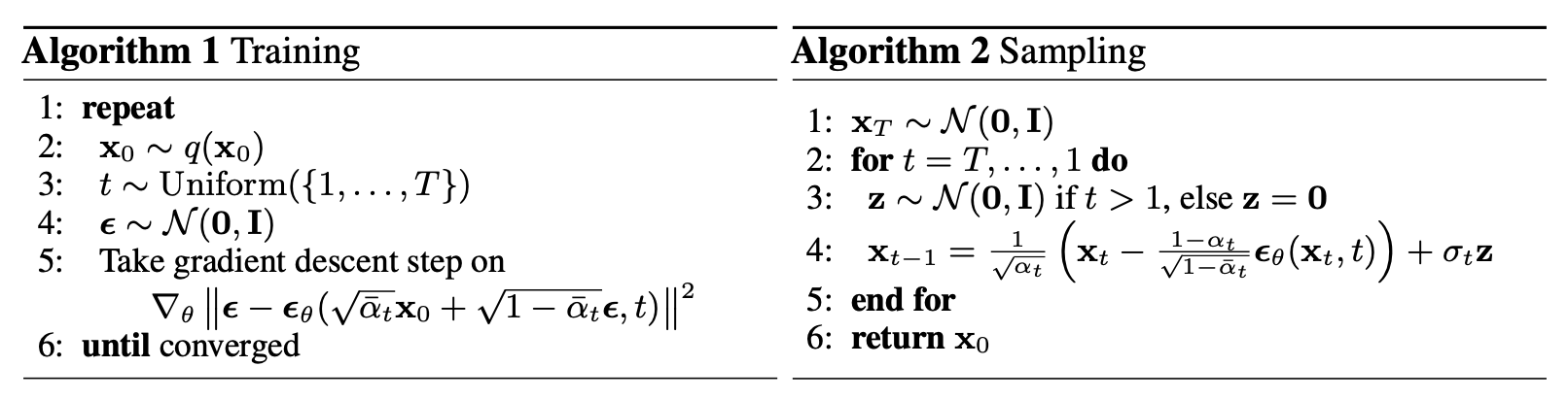 Fig. 2. Training and sampling algorithm. (Source: Ho et al. 2020)
Generated Samples
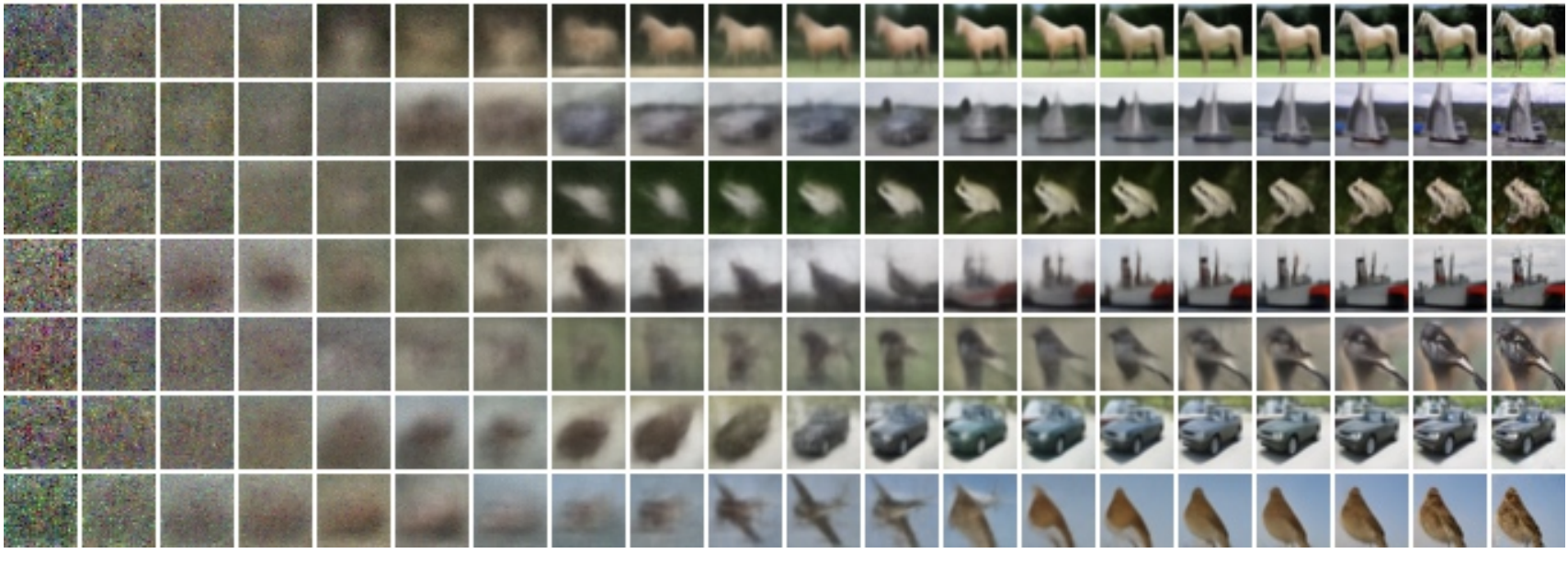 Fig. 3. Unconditional CIFAR10 progressive generation. (Source: Ho et al. 2020)
Lecture Note Version
You can download the lecture note version!
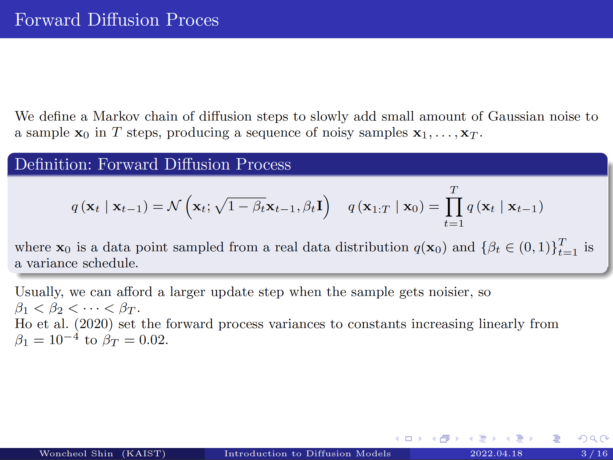 Fig. 4. Example slide 1
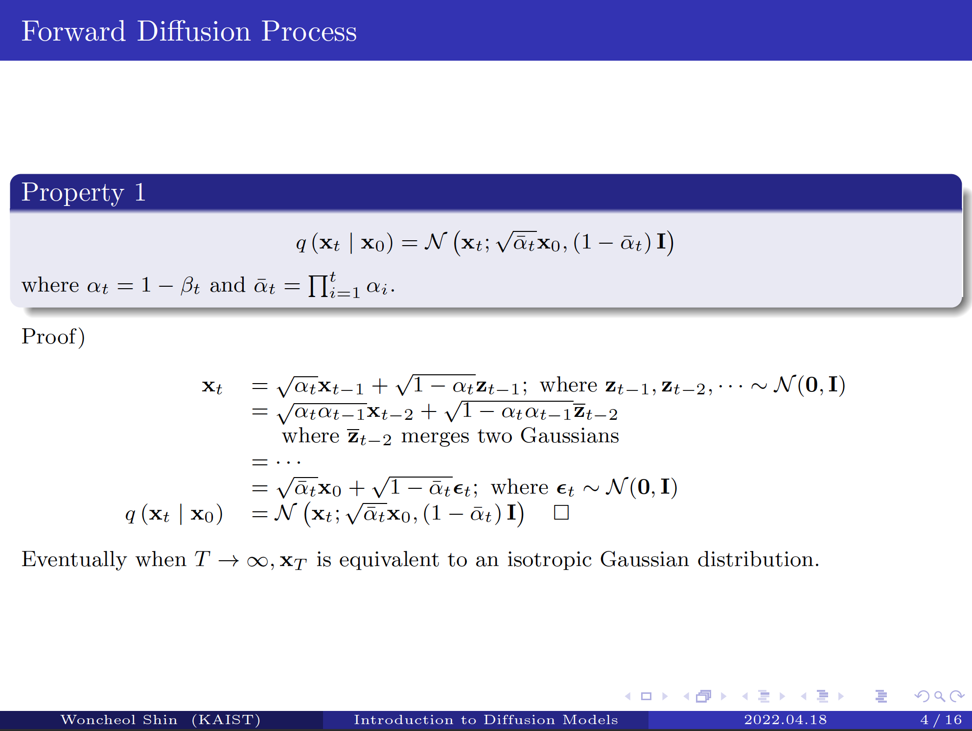 Fig. 5. Example slide 2
References
[1] Weng, Lilian. (Jul 2021). What are diffusion models? Lil’Log. https://lilianweng.github.io/posts/2021-07-11-diffusion-models/.
[2] Jonathan Ho et al. “Denoising diffusion probabilistic models.” arxiv Preprint arxiv:2006.11239 (2020).
Citation
Shin, Woncheol. (April 2022). Introduction to Diffusion Models Shin’s Blog. https://wcshin-git.github.io/2022/04/18/Intro_Diffusion.html.
Or
@article{shin2022intro,
  title   = "Introduction to Diffusion Models",
  author  = "Shin, Woncheol",
  journal = "wcshin-git.github.io",
  year    = "2022",
  month   = "April",
  url     = "https://wcshin-git.github.io/2022/04/18/Intro_Diffusion.html"
}