Introduction to Cell Annotation with ScType
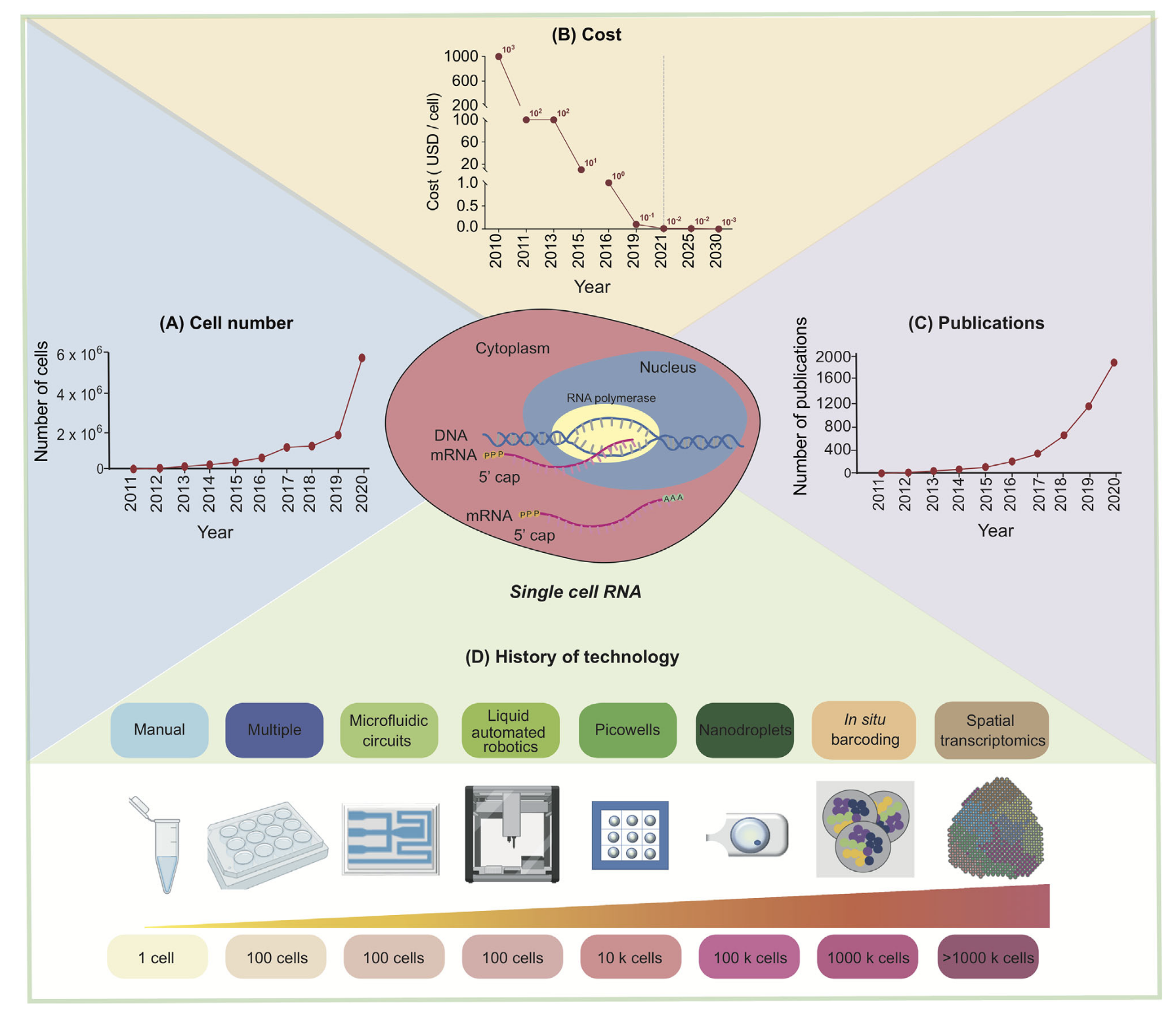 Fig. Development of single-cell RNA sequencing technology. (Source: Jovic et al. 2021)
Single-cell RNA sequencing (scRNA-seq) has revolutionized the fields of biology and medicine by enabling exploration of the transcriptomic profiles of individual cells.
This post aims to show how to use ScType to annotate cells in R code.
This post can be divided into two main parts:
1) Clustering Tutorial, which covers selecting cells (quality control), normalizing the data, identifying highly variable features, scaling the data, performing PCA, clustering the cells, and visualizing the clusters using UMAP.
2) Cell Annotation using ScType.
1. Clustering Tutorial
Download the example dataset and code
Run git clone or click this link to download.
git clone https://github.com/wcshin-git/Cell_Annotation_with_ScType
Import the required packages
lapply(c("dplyr","Seurat","HGNChelper","openxlsx"), library, character.only = TRUE)
If any of the packages are missing, please install them first.
Load the example dataset
pbmc.data <- Read10X(data.dir = "filtered_gene_bc_matrices/hg19")
# (32738, 2700)
we will analyze the dataset of Peripheral Blood Mononuclear Cells (PBMC) freely available from 10X Genomics. There are 2,700 single cells that were sequenced on the Illumina NextSeq 500.
Let’s examine pbmc.data by looking at a few genes in the first 30 cells.
pbmc.data[c("CD3D", "TCL1A", "MS4A1"), 1:30]
3 x 30 sparse Matrix of class "dgCMatrix"

CD3D  4 . 10 . . 1 2 3 1 . . 2 7 1 . . 1 3 . 2  3 . . . . . 3 4 1 5
TCL1A . .  . . . . . . 1 . . . . . . . . . . .  . 1 . . . . . . . .
MS4A1 . 6  . . . . . . 1 1 1 . . . . . . . . . 36 1 2 . . 2 . . . .
The . values in the matrix represent 0s. Since most values in an scRNA-seq matrix are 0, Seurat uses a sparse-matrix representation whenever possible.
Setup the Seurat Object
pbmc <- CreateSeuratObject(counts = pbmc.data, project = "pbmc3k", min.cells = 3, min.features = 200)
# Retain genes expressed in at least 3 cells and cells with at least 200 detected genes.
# (13714, 2700)
The object serves as a container that contains both data (like the count matrix) and analysis (like PCA, or clustering results) for a single-cell dataset.
Quality Control
# percentage of counts originating from a set of mitochondrial genes
pbmc[["percent.mt"]] <- PercentageFeatureSet(pbmc, pattern = "^MT-")
Low-quality / dying cells often exhibit extensive mitochondrial contamination.
# Visualize QC metrics as a violin plot
VlnPlot(pbmc, features = c("nFeature_RNA", "nCount_RNA", "percent.mt"), ncol = 3)
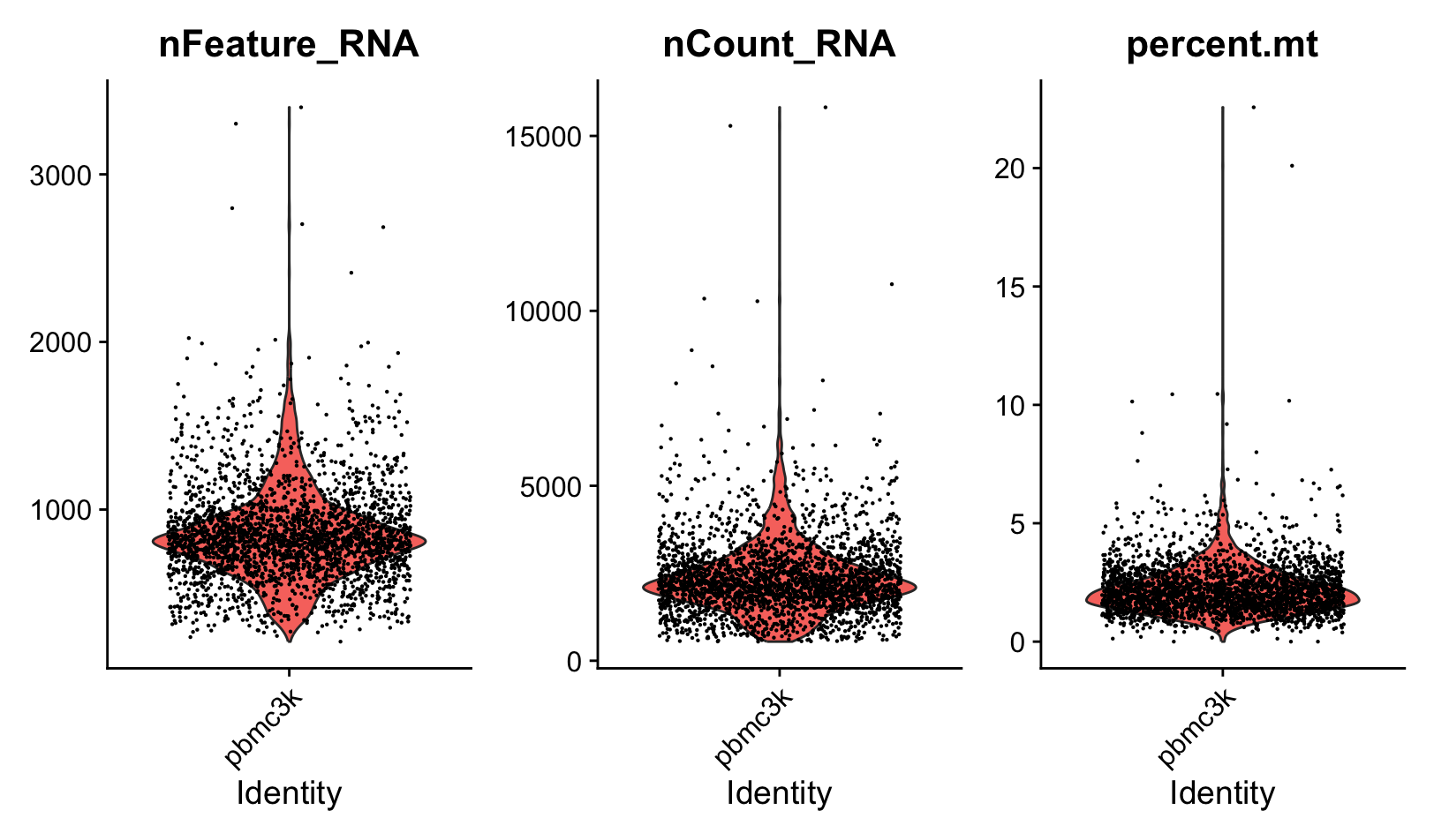
nFeature_RNA represents the number of unique genes (features) detected in each cell. nCount_RNA represents the total number of RNA molecules detected in each cell.
# Cell filtering
pbmc <- subset(pbmc, subset = nFeature_RNA > 200 & nFeature_RNA < 2500 & percent.mt < 5)
# (13714, 2638)
Low-quality cells or empty droplets will often have very few genes. Cell doublets or multiplets may exhibit an aberrantly high gene count.
Normalize data
pbmc <- NormalizeData(pbmc, normalization.method = "LogNormalize", scale.factor = 10000)
“LogNormalize” normalizes the feature expression measurements for each cell by the total expression, multiplies this by a scale factor, and log-transforms the result.
Identification of highly variable features
pbmc <- FindVariableFeatures(pbmc, selection.method = "vst", nfeatures = 2000)
Focusing on these genes in downstream analysis helps to highlight biological signal in single-cell datasets.
Scaling the data
pbmc <- ScaleData(pbmc, features = rownames(pbmc))
Shifts the expression of each gene, so that the mean expression across cells is 0.
Scales the expression of each gene, so that the variance across cells is 1.
Run PCA
pbmc <- RunPCA(pbmc, features = VariableFeatures(object = pbmc))
Perform PCA on the scaled data for dimensional reduction.
# Check number of PC components
ElbowPlot(pbmc, ndims=20)
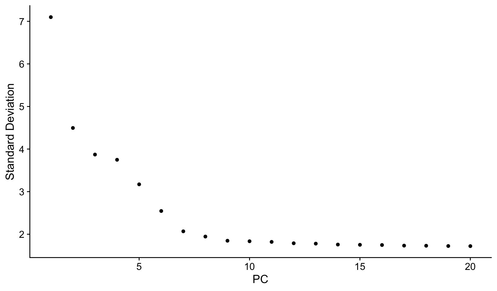
We will select 10 PCs for downstream analysis, based on Elbow plot.
Cluster and visualize
pbmc <- FindNeighbors(pbmc, dims = 1:10)
pbmc <- FindClusters(pbmc, resolution = 0.5)
pbmc <- RunUMAP(pbmc, dims = 1:10)
DimPlot(pbmc, label = TRUE, reduction = "umap")
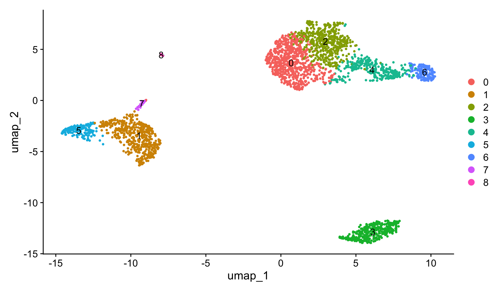
The resolution parameter in FindClusters() sets the ‘granularity’ of the downstream clustering, with increased values leading to a greater number of clusters.
2. Cell Annotation
Now, let’s annotate the clusters with known cell types using ScType.
Load required functions
# load gene set preparation function
source("https://raw.githubusercontent.com/IanevskiAleksandr/sc-type/master/R/gene_sets_prepare.R")
# load cell type annotation function
source("https://raw.githubusercontent.com/IanevskiAleksandr/sc-type/master/R/sctype_score_.R")
Prepare marker gene sets
# DB file
db_ <- "https://raw.githubusercontent.com/IanevskiAleksandr/sc-type/master/ScTypeDB_full.xlsx";
tissue <- "Immune system" # e.g. Immune system,Pancreas,Liver,Eye,Kidney,Brain,Lung,Adrenal,Heart,Intestine,Muscle,Placenta,Spleen,Stomach,Thymus

# prepare gene sets
gs_list <- gene_sets_prepare(db_, tissue)
Run ScType
# check Seurat object version (scRNA-seq matrix extracted differently in Seurat v4/v5)
seurat_package_v5 <- isFALSE('counts' %in% names(attributes(pbmc[["RNA"]])));
print(sprintf("Seurat object %s is used", ifelse(seurat_package_v5, "v5", "v4")))

# extract scaled scRNA-seq matrix
scRNAseqData_scaled <- if (seurat_package_v5) as.matrix(pbmc[["RNA"]]$scale.data) else as.matrix(pbmc[["RNA"]]@scale.data)

# run ScType
es.max <- sctype_score(scRNAseqData = scRNAseqData_scaled, scaled = TRUE, gs = gs_list$gs_positive, gs2 = gs_list$gs_negative)
The score is calculated through the following process:
1) Z-score Standardization
For each gene (row), the expression values across multiple cells (columns) are standardized using the z-score.
2) Calculating and Applying Marker Sensitivity
Genes that appear as markers for multiple cell types are given scores closer to 0, while those that are more specific to a single cell type receive scores closer to 1. By multiplying the z-scored expression matrix by these sensitivity scores, we effectively weight each gene according to how important it is for distinguishing that particular cell type.
3) Cell-Type Scoring via Positive/Negative Markers
For a given cell, the expression values (already multiplied by the gene-specificity scores) of the positive marker genes for a particular cell type are summed. To reduce biases due to varying numbers of marker genes, the total is divided by the square root of the number of marker genes. Negative markers for that cell type are also summed, but with a negative sign, and added in. The final value represents the score of that cell for that specific cell type.
Assigning Cell Types to Clusters
# merge by cluster
cL_resutls <- do.call("rbind", lapply(unique(pbmc@meta.data$seurat_clusters), function(cl){
    es.max.cl = sort(rowSums(es.max[ ,rownames(pbmc@meta.data[pbmc@meta.data$seurat_clusters==cl, ])]), decreasing = !0)
    head(data.frame(cluster = cl, type = names(es.max.cl), scores = es.max.cl, ncells = sum(pbmc@meta.data$seurat_clusters==cl)), 10)
}))
sctype_scores <- cL_resutls %>% group_by(cluster) %>% top_n(n = 1, wt = scores)

# set low-confident (low ScType score) clusters to "unknown"
sctype_scores$type[as.numeric(as.character(sctype_scores$scores)) < sctype_scores$ncells/4] <- "Unknown"
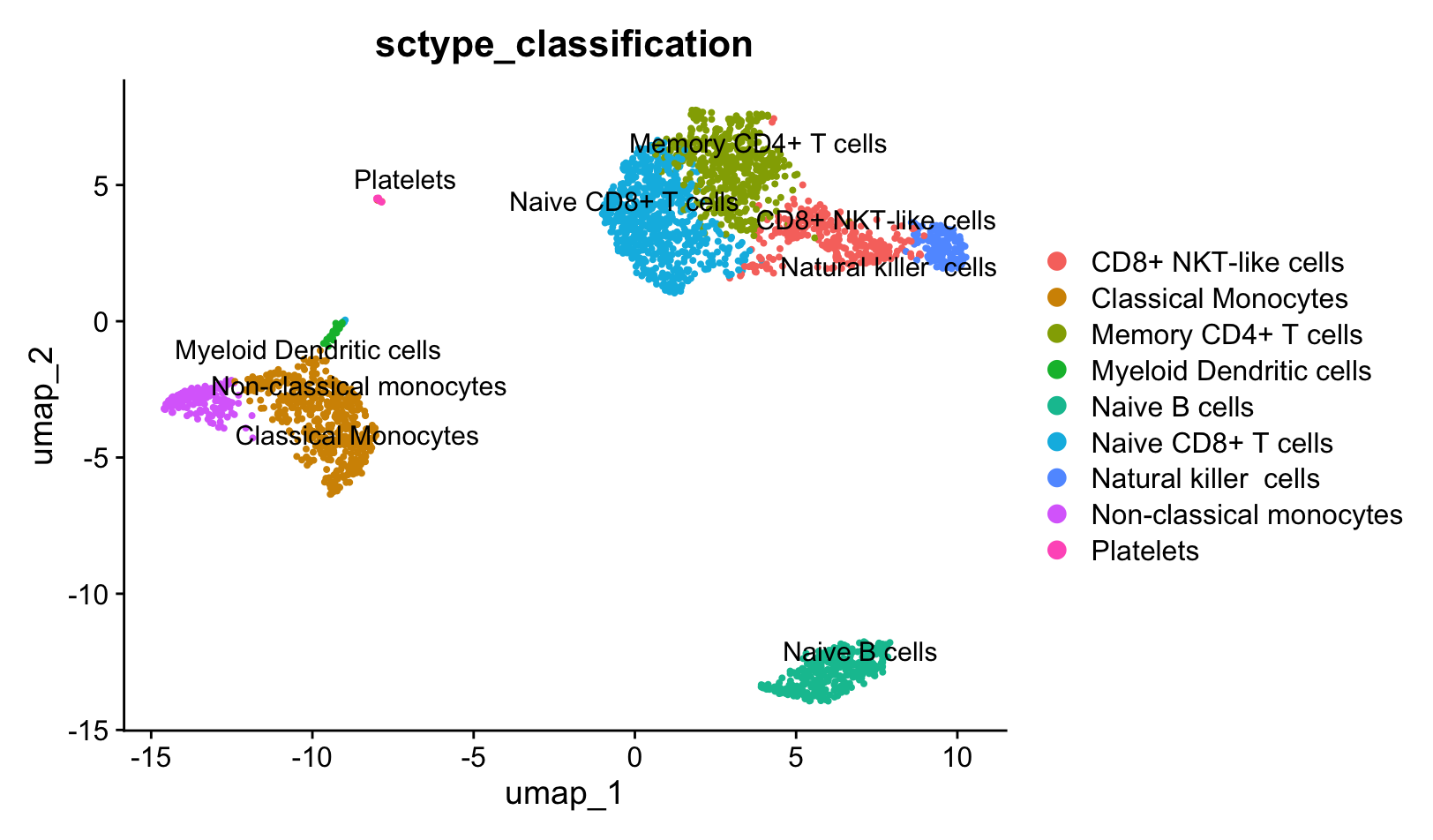
We sum the ScType scores of the cells within each cluster and select the cell type with the highest score for each cluster.
Visualization
pbmc@meta.data$sctype_classification = ""
for(j in unique(sctype_scores$cluster)){
  cl_type = sctype_scores[sctype_scores$cluster==j,];
  pbmc@meta.data$sctype_classification[pbmc@meta.data$seurat_clusters == j] = as.character(cl_type$type[1])
}

DimPlot(pbmc, reduction = "umap", label = TRUE, repel = TRUE, group.by = 'sctype_classification')
References
[1] Jovic, Dragomirka, et al. “Single‐cell RNA sequencing technologies and applications: A brief overview.” Clinical and translational medicine 12.3 (2022).
[2] Ianevski, Aleksandr, Anil K. Giri, and Tero Aittokallio. “Fully-automated and ultra-fast cell-type identification using specific marker combinations from single-cell transcriptomic data.” Nature communications 13.1 (2022)
[3] https://github.com/IanevskiAleksandr/sc-type
[4] https://satijalab.org/seurat/articles/pbmc3k_tutorial#determine-the-dimensionality-of-the-dataset
[5] http://youtube.com/watch?v=huxkc2GH4lk